Introduction

Calculating volumes of earth, aggregate or holes over varying terrain is a challenging mathematical task that can have a huge impact on project budgets or predicted revenue. It is a relatively simple process that can be performed with free and open source software in a few simple steps. All that is required is elevation data from LiDAR or UAV photogrammetry in the form of point clouds which can then be converted into a Digital Elevation Model (DEM)/Digital Surface Model (DSM) as per this tutorial.
Some applications for these volume calculations are finding how much material is needed to fill a hole, how much volume will be extracted by mining an area to a certain depth, how much volume is in a pile of aggregate or finding how much material has been removed from an area.

The following is an advanced method tutorial that takes a step by step approach to answering these questions by using QGIS tools and elevation data from LiDAR and from UAVs/Drones to calculate volumes with centimeter precision. A simplified approach can be found here. By following these 10 steps, you will be able to create a volume estimate from a LiDAR/UAV point cloud or a DEM.

Step 1. Identify Volume Feature
Step 2. Create Clip Feature Layer
Step 3. Digitize Clip Area
Step 4. Add Clip Area Z-Values
Step 5. Create Interpolated Surface (TIN)
Step 6. Clip TIN Surface
Step 7. Calculate Elevation Change
Step 8. Calculate Zonal Statistics
Step 9. Calculate Zone Volumes
Step 10. Calculate Total Volume

Calculate Surface from Baseline Elevation

Calculate Volume from Interpolated/Best Fit Surface.

Step 1.

After opening a new QGIS project, we will start by importing a DEM/DSM raster into the map. If you need to create a surface follow our tutorial on how to create a DEM from LiDAR tutorial here.
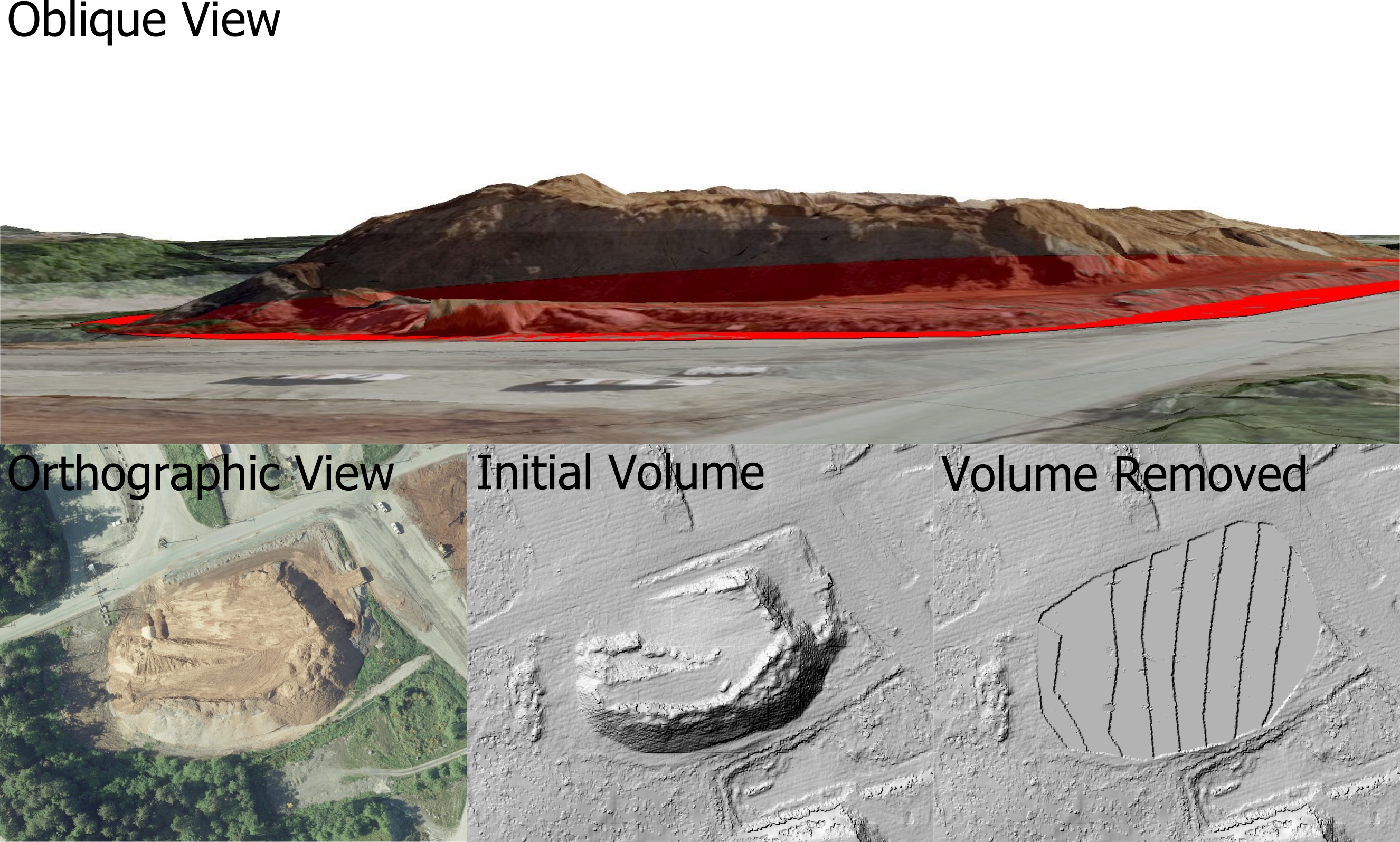
This surface should have a terrain feature with significant rise or constrained depth/hole over which a volume can be calculated. A section of sloped terrain can also be used for combining cut/fill volumes for leveling a section of ground.
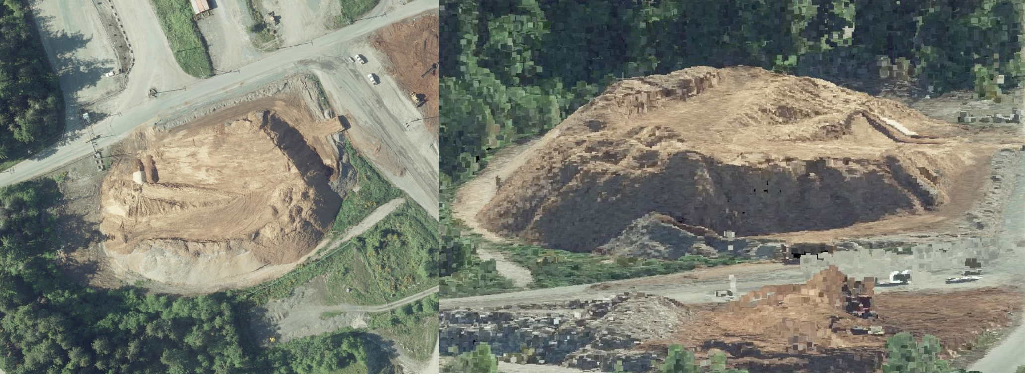
The gravel pile in the image below is our target area. We want to know how many truck loads of gravel are in the stock pile.

Target Volume Area - Aggregate Pile

Step 2. Create Clip Feature Layer

We want to limit the DEM area for the Volume Calculations to make the results as accurate as possible. This requires creating a new polygon area to clip the DEM raster to.
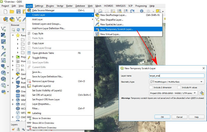
With QGIS create a "New Temporary Scratch Layer" from the Layer menu bar. Then from Create Layer select New Temporary Scratch Layer.
A new window will popup with settings for the temporary layer. Enter in a unique layer name, select a MutiPolygon/MultiSurface Geometry Type and ENSURE that the Spatial Reference System is the same as the DEM raster.

Step 3. Digitize Clip Area

With an empty polygon layer established we will now digitize the target area. Try to select edge directly at the base of the feature. Having high resolution imagery helps as well as a hillshade version of the DEM. Alternate between the two rasters to ensure the most accurate volumes possible.

Step 4. Add Z-Values to Clip Layer

We are now going to add elevation values to the clip area we just created. By doing this we will be able to estimate what the terrain will look like after the volume has been removed.
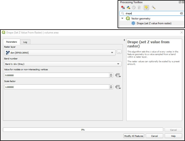
This is a quick and easy process with QGIS and an existing DEM. Start by right clicking on the clip layer and select Toggle Editing from the popup menu. Now open the Processing Toolbox and search for "Drape (set Z value from raster). We can add the Z values without creating a new layer by selecting the "Edit Features In-Place" option at the top of the Processing Toolbox panel. Open the Drape (set Z value from raster) toolbox and select the DEM/DSM as the "Raster Layer". Leave the rest of the settings as default.

Step 5. Create Interpolated Surface

The interpolated surface will represent what the terrain will look like after the volume is removed. We are assuming that the volume is not located on flat terrain and once the volume is removed the slope of underlying are will be similar to the area surrounding the clip area. Otherwise we can use the simplified method using a constant base elevation.
We are going to use the Triangulated irregular Network (TIN) method to calculate a base elevation raster. This method will create a base surface that has been averaged across the edges of the clip area resulting in a smooth transition from the high elevation sides to the lower elevation sides.

So, to create our base surface we will activate the clip area polygon layer (if the layer is active it will automatically be entered as the input layer when the processing tool is opened) and then go back to the Processing Toolbox and search for the "TIN interpolation" tool.
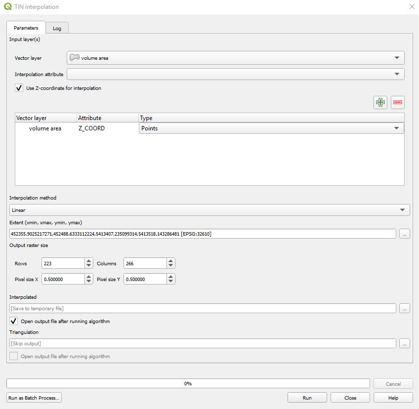
The inputs for the TIN Interpolation should be as follows:
Input Layer(s): enter your clip area layer name here
Use Z-coordinate for interpolation: AND (click plus button to add Z_COORD as interpolation attribute)
Interpolation Method: Linear
Extent: Click on ellipses -> use layer extent -> (select your clip area layer)
Output raster size: Enter x/y pixel size of your DEM/DSM raster (look in layer properties if you are unsure of the resolution)
We will have to do some further manipulations to this layer, so we can leave it as a [Save to temporary file] layer to reduce data clutter.

Step 6. Clip TIN Surface to Clip Area Polygon

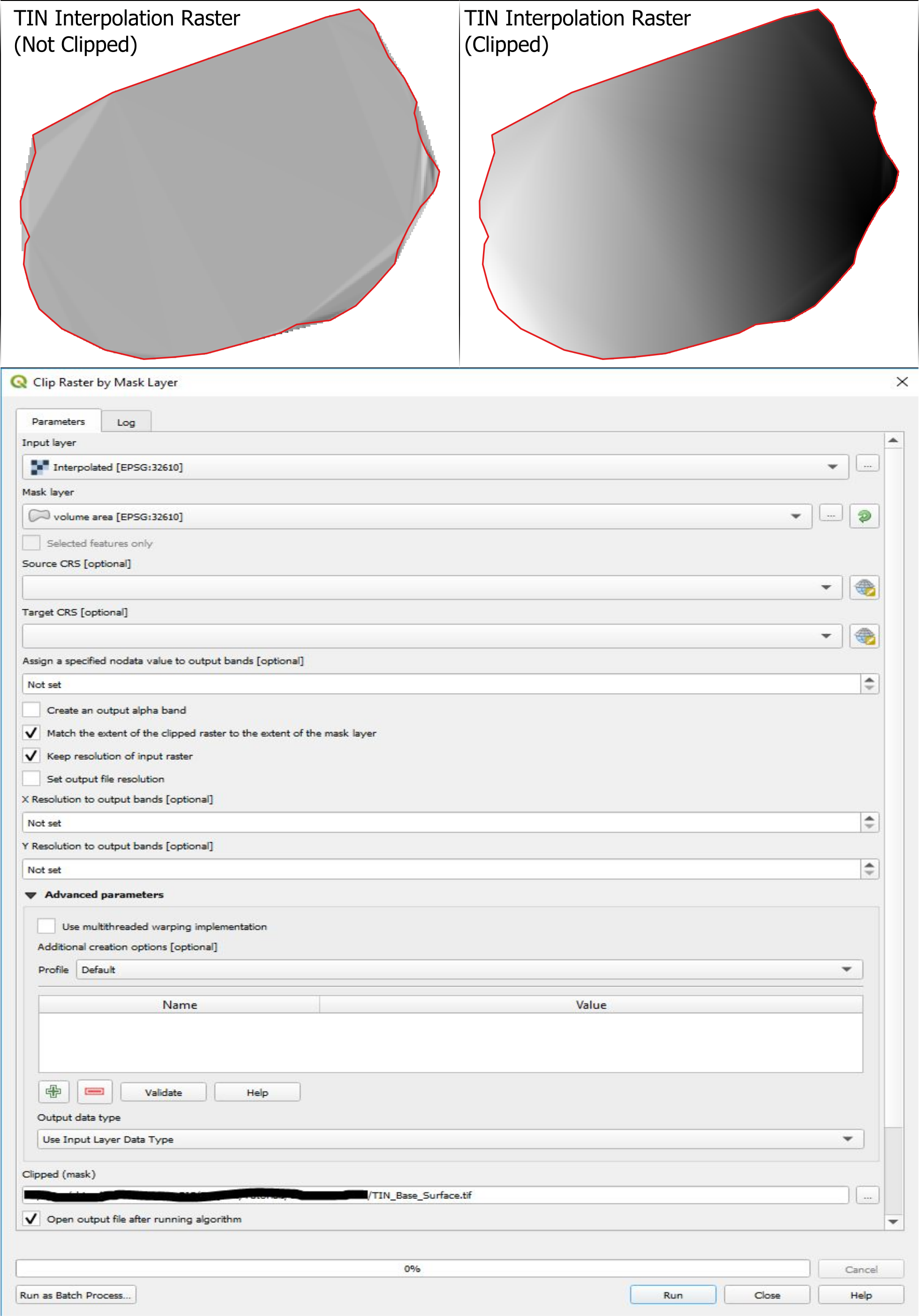
Depending on how irregular our clip area is, the resulting TIN Interpolation may produce a raster that goes beyond the boundary of our target area. To ensure we only perform a volume calculation on our digitized area, we willclip the TIN Interpolation Raster to the digitized polygon area.
To do this we will select/activate the new TIN Interpolated raster in the TOC then go back to the Processing Toolbox and search for "Clip raster by mask layer". The input values should be as follows:
Input Layer: TIN Interpolated Raster
Mask Layer: Clip Area Polygon Layer
Keep resolution of input raster:
Clipped (mask): //path/to/project/folder/output_name.tif
Open output file after running algorithm:

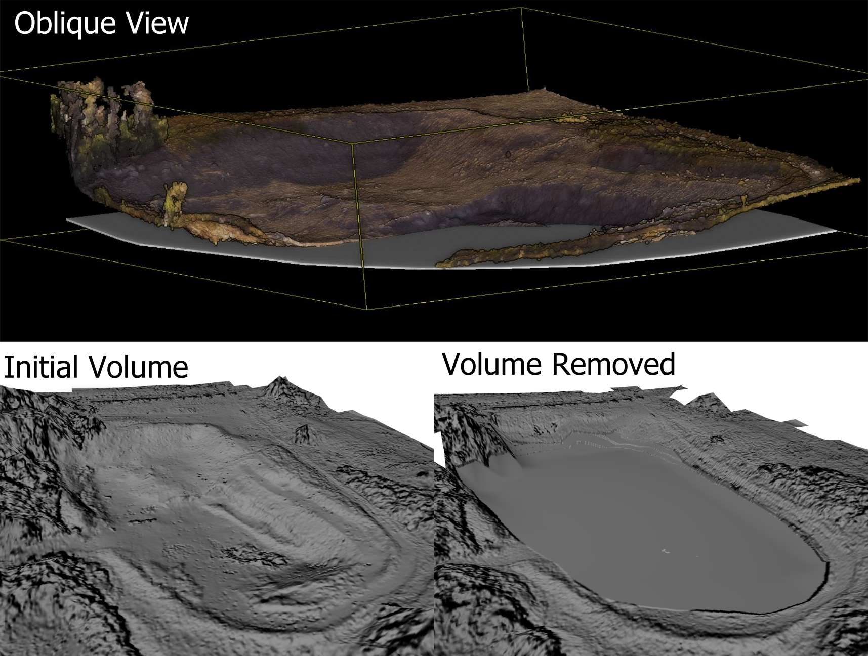
Step 7. Calculate Elevation Change

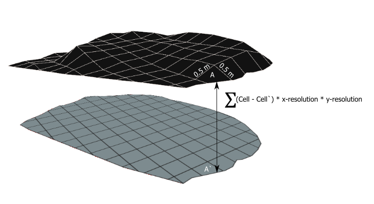
The volume that we are about to calculate is essentially the relative difference between the DSM/DEM and the TIN surface we generated (this step). Then for each raster cell, using a zonal statistics tool (Step 8) and the Field Calculator (Step 9), we will multiply the difference by the area of each cell (i.e. a difference of 8 meters in elevation for a 0.5 m² or 0.5 m resolution raster cell will be 2 m³ volume) and then sum the value of all the raster cells together for a total volume (See Step 10).

Volume Calculation Diagram/Equation

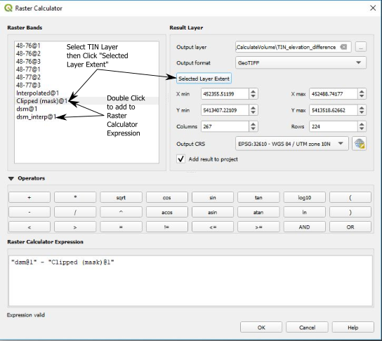
Using the QGIS Raster Calculator from the QGIS Raster drop down menu, we will subtract the TIN Interpolated surface from the DEM/DSM creating a new raster layer.

Step 8. Zonal Statistics

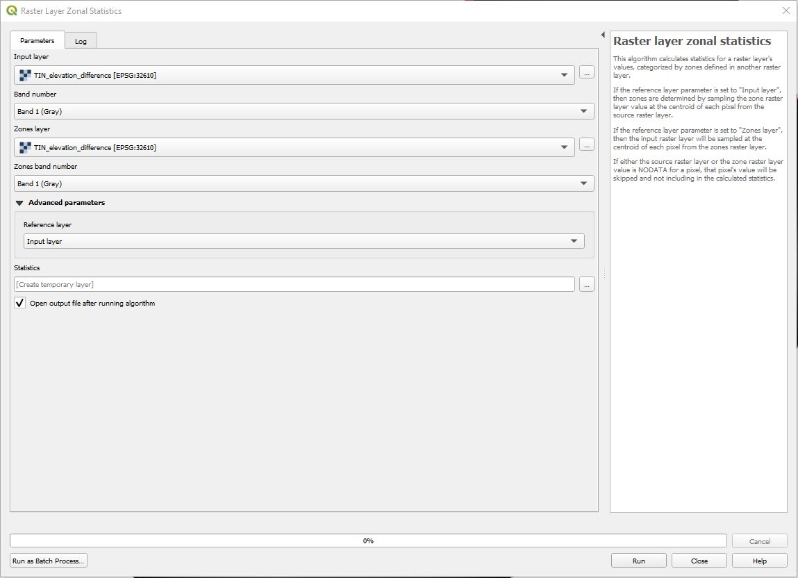
Now that we know the relative difference in height for each raster pixel, we can use the Raster layer zonal statistics tool to calculate the cell areas and sum of the elevation difference values. This will essentially result in a table where identical raster cell values have been grouped and summarized, in our case elevation difference values.

The Raster layer zonal statistics tool can be found by searching for it in the Processing Toolbox. Use the raster output from the raster calculator as the Input Layer for this tool. For the output, I prefer to leave the results as a temporary layer because we are only interested in the summary statistics of the results.

Step 9. Calculate Zone Volumes with Field Calculator

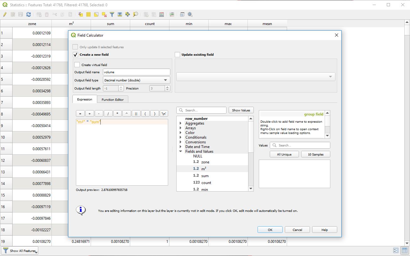
The resulting layer from the Raster Zonal Statistics was a new table with statistics and summaries for each raster zone (i.e. group of raster cells with the same value). Right click on the zonal statistics table in the Layers Panel an select Open Attributes Table. The table might take a minute to open depending on the size of your volume area and the resolution of the DEM. Take a moment to view some of the values in the table and look at the field names to see what zonal statistics have automatically been calculated.
We are mainly interested in the zone, m², sum and count. The zone field is the difference in elevation value that was calculated using the raster calculator. m² is the area of the zone and sum is the total elevation difference for all the cells/pixels in that specific zone. To find a volume for each zone we will need to multiply the sum field and the m² field using the Field Calculator to create a new field with a volume calculated for each zone.
Click on the Abacus icon at the top of the table or use the control-i command to open the field calculator. Create a new field with the Output field name as volume the Output field type as Decimal number (double) ***this value may be different if your table was saved in a different format. In the field expression enter "m^²" * "sum" and then click OK.
A new field will now be visible in the table that represents the volume of each zone.

Step 10. Calculate Total Volume

The final step to finding our volume is to summarize the zonal statistics table based on the volume field that we calculated in the last step.
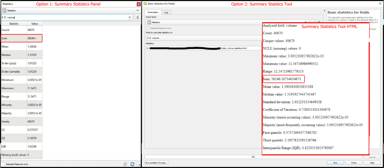
QGIS has two quick options for doing the summary. The first is using the Statistics Panel. You can find the panel by going to the View -> Panels -> Statistics menu at the top of the screen. There is a drop down menu within the Statistics Panel where we can select the Zonal Statistics table from the previous step and then select the volume field to see the summary statistics. The total volume is represented by the Sum Statistic.
The second way to find the total volume is to use the Basic Statistics for fields tool that will create an HTML file with the summary statistics where the Sum statistic will represent the total volume.

Conclusion

There you have it! Using free and open source software we were able to accurately measure the volume of a surface feature in 10 easy steps.
There are many advantages to using this method. It gives you fine grain control over the calculations and clip area. It is remarkably processing efficient and cost effective as the software is free. The whole process can be automated for a one or two click solution (a topic for a future blog).
I have used this method frequently when calculating volumes and areas for our mining and construction clients. We have had great success with our estimates and have similar results when compared to expensive software from ESRI or Pix4D photogrammetry software, with the added benefit of being able to customize the base surface to suit the need of the customer and the project type.
Hopefully you found this tutorial useful. Please feel free to leave your comments below by securely logging in with your GitHub, Twitter or Facebook account or send us an email.