LiDAR Digital Elevation Model (DEM) using QGIS and GRASS GIS
Overview
Modeling terrain is a powerful function of a GIS. With the emergence of Airborne LiDAR, being able to turn the millions of highly accurate laser point readings into a surface that can be used to perform analysis on a large scale is invaluable.
As LiDAR data becomes more accessible, many industries and consultants will be able to utilize the data for analysis. It seems, however, that many people shy away from using LiDAR or do not use LiDAR to its full potential due to lack of experience in working with the data or the assumption that the cost of the data is too expensive or the cost of the software required to process it is too complicated or too expensive as well.
As a first step in breaking down the accessibility barriers to LiDAR, this article will walk through the common task of creating a Digital Elevation Model (DEM) or more specifically a Digital Surface Model (DSM) which is a raster/image/gridded representation of the ground topography with the vegetation and buildings removed. The DEM/DSM is the base data that can be used in many types of environmental and terrain modeling such as calculating watersheds, flood areas, viewsheds, slopes and terrain feature identification. In order to accomplish this we will use QGIS 3.4 which has access to the GRASS GIS 7.4 tools.
There are several ways to process LiDAR with free and open source solutions. I like using this method because all of the processing, analysis, visualization and mapping can be done with one environment. This is adventitious as analysis becomes more complicated at which point you can start creating scripts and tools to automate a lot of the time consuming and repetitive processes (a topic for a future tutorial). QGIS is ideal because comes with GRASS tools integrated into it (possibly not for macOS)
The data set we will use for this tutorial is from Open Topography and is available at this link.
Open Topography is an awesome source for elevation information numerous reasons. Not only does it provide LiDAR data at no cost but it will provide you with many of the computationally intensive elevation products, such as Hillshades, DEMs, Point Cloud Viewer and much much more!
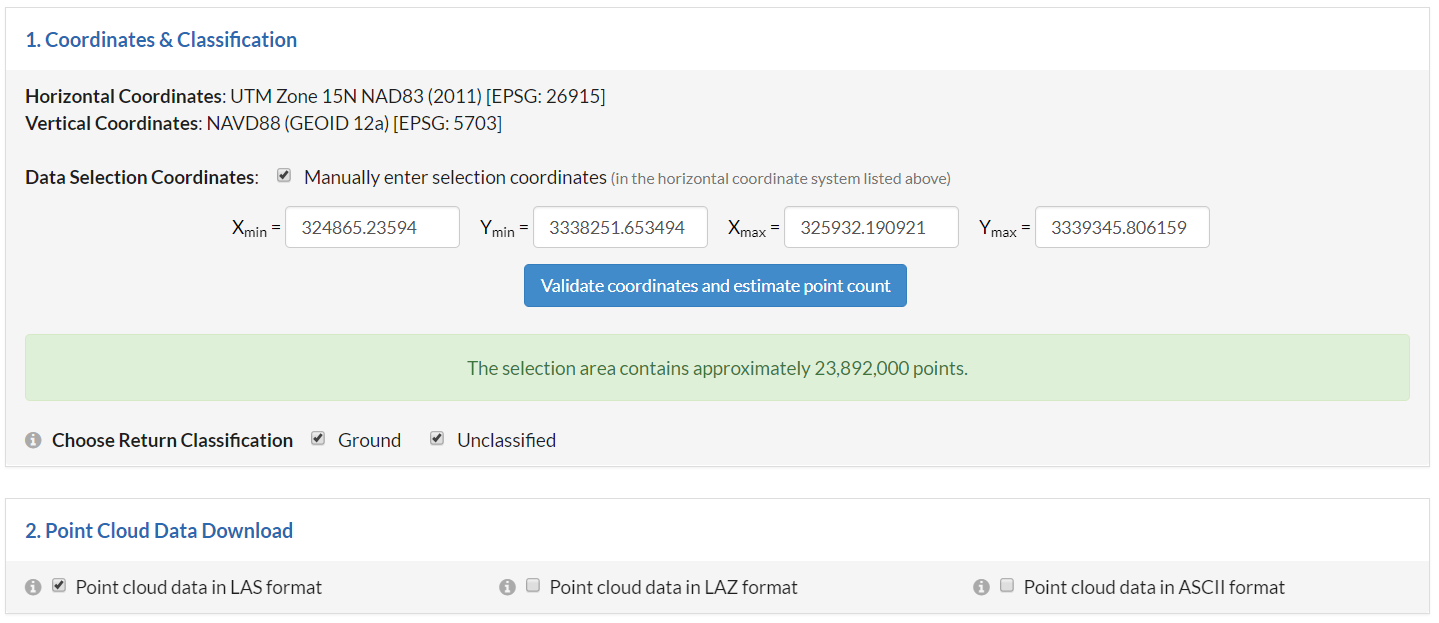
However, for the purpose of this tutorial we will choose to download only a small portion of the LiDAR data, unselecting all of the other options that Open Topography provides.
The image below shows the parameters used to download that LiDAR data be sure to select .las format!
Step 1
Inspect the LiDAR metadata to find out what Spatial Reference System (SRS) the LiDAR data is in, to get an idea of how any points per square meter there are on average and see how the LiDAR data has been classified (i.e. ground returns and non-ground returns). To get a better understanding of how LiDAR data is structured take a look at the GISGeography website has an excellent description of how LiDAR works and ASPRS - The Imaging and Geospatial Information Society has set the standard for how LiDAR should be classified.
Below is the meta data that can be downloaded along with the point cloud data from Open Topography. The most important details to note at this point is the horizontal and vertical coordinate systems (specifically the EPSG codes).
Dataset Information:

Dataset Name: Trinity River, Texas 2015
Dataset Short Name: TX15Passalacqua
DOI: 10.5069/G9JW8BX4

Acknowledgement:
LiDAR data acquisition and processing completed by the National Center for Airborne Laser Mapping (NCALM). NCALM funding provided by NSF's Division of Earth Sciences, Instrumentation and Facilities Program. EAR-1339015.Passalacqua, P. (2015): Trinity River, Texas 2015 airborne lidar. National Center for Airborne Laser Mapping (NCALM), distributed by OpenTopography.
https://doi.org/10.5069/G9JW8BX4

Data Access Acknowledgement: This material is based on [data, processing] services provided by the OpenTopography Facility with support from the National Science Foundation under NSF Award Numbers 1226353 & 1225810

Horizontal Coordinates: UTM Zone 15N NAD83 (2011) [EPSG: 26915]
Vertical Coordinates: NAVD88 (GEOID 12a) [EPSG: 5703]

Job Description:
	User:[Guest] zking03@hotmail.com
	Job ID: pc1547927335266
	Title: Trinity River, Texas 2015 - Practice
	Description:This LiDAR data set is intended for practicing how to generate elevation products over forested terrain.

Job Processing Result:
	Submission Time: 2019-01-19 11:48:55
	Completion Time: 2019-01-19 11:49:35
	Duration: 40 seconds
	Number of Points: 23,787,091
	Status: Done

Data Selection Coordinates:
	Xmin: 324865.23594
	Xmax: 325932.190921
	Ymin: 3338251.653494
	Ymax: 3339345.806159
	Classifications: all

Point Cloud Results:
	Download point cloud data in ASCII format: No
	Download point cloud data in LAS format: Yes
	Download point cloud data in LAZ format: No

DEM Generation (Local Gridding):
	Calculate Zmin grid: No
	Calculate Zmax grid: No
	Calculate Zmean grid: No
	Calculate Zidw grid: No
	Calculate point count: No

DEM Generation (TIN):
	Calculate TIN: No

Derivative Products:
	Generate Hillshades & Slopes: N/A

Visualization:
	Images & Google Earth KML: No

3D Point Cloud Visualization: No
Hydrologic Terrain Analysis (TauDEM) Products:
	Hydrologically correct DEM with pits filled: No
	D-Infinity Flow Direction : No
	D-Infinity Specific Catchment Area: No
	Topographic Wetness Index: No
	D8 Flow Direction: No
	tauDemD8FlowDir: No
SOL Products:
	sol: No
Step 2
In this next step we will use some statistics go gain a little more insight into the point cloud data. Our goal is to see what what we can use as a maximum resolution for our DEM. To do this we will calculate how many LiDAR ground points there are per square meter using GRASS GIS' r.in.lidar tool and the built in QGIS Raster Information... tool.
Open a new QGIS project (download and install a free copy now if you have not done so already! Once the program is open make sure you set the default spatial reference system/projection/EPSG to match that of the LiDAR dataset. Next, click on the gear shaped "Toolbox" button in the tool bar to open the "Processing Toolbox". In the search box enter r.in.lidar
The key parameters to enter into the tool are:
LAS input file=points.las
Statistics to use for raster values=n (i.e. number of lidar points per raster cell)
Storage type for resultant raster map=CELL
Filter range for z data=-10000, 10000 (use large values to ensure all points fall within the range)
Filter range for intensity values=-10000, 10000
Output raster resolution=1
Only import points of selected class(es)=2
Lidar Raster=/output/file/path/lidar_density.tif
Advanced parameters
Use the extent of the input for the raster extent=Checked
Set the computation region to match the new raster map=Checked
Override projection check=Checked

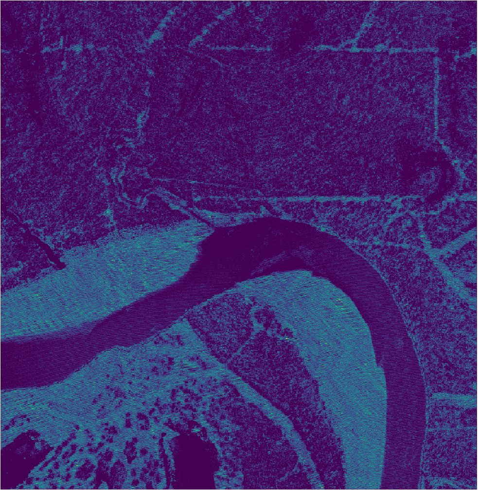
The output raster should look similar to the image below and at first look will not give us much information. In step 3 we will perform some simple statistics on this raster to help us choose the optimal resolution for our elevation products.
Step 3
Using the built in QGIS Raster Information... tool. The tool is located in the drop-down menu at the top of the QGIS window: Raster -> Miscellaneous -> Raster Information...
Using the raster generated in Step 2 as the input layer, with Force computation of the actual min/max values for each band checked and Read and display image statistics (force computation if necessary) checked we will compute the raster statistics.
The tool will output a .html file that should be saved along with the other outputs and data from this tutorial for future reference.
A snippet of the output can be seen below
Driver: GTiff/GeoTIFF
Files: //file/path/Texas-TrinityRiver/point-density.tif
//file/path/Projects/Texas-TrinityRiver/point-density.tif.aux.xml
Size is 1068, 1095
Coordinate System is:
PROJCS["UTM Zone 15, Northern Hemisphere",
GEOGCS["grs80",
DATUM["unknown",
SPHEROID["Geodetic_Reference_System_1980",6378137,298.257222101],
TOWGS84[0,0,0,0,0,0,0]],
PRIMEM["Greenwich",0],
UNIT["degree",0.0174532925199433]],
PROJECTION["Transverse_Mercator"],
PARAMETER["latitude_of_origin",0],
PARAMETER["central_meridian",-93],
PARAMETER["scale_factor",0.9996],
PARAMETER["false_easting",500000],
PARAMETER["false_northing",0],
UNIT["metre",1,
AUTHORITY["EPSG","9001"]]]
Origin = (324865.000000000000000,3339346.000000000000000)
Pixel Size = (1.000000000000000,-1.000000000000000)
Metadata:
AREA_OR_POINT=Area
TIFFTAG_SOFTWARE=GRASS GIS 7.4.2 with GDAL 2.3.2
Image Structure Metadata:
COMPRESSION=LZW
INTERLEAVE=BAND
Corner Coordinates:
Upper Left ( 324865.000, 3339346.000) ( 94d49' 7.91"W, 30d10'22.58"N)
Lower Left ( 324865.000, 3338251.000) ( 94d49' 7.26"W, 30d 9'47.02"N)
Upper Right ( 325933.000, 3339346.000) ( 94d48'28.00"W, 30d10'23.13"N)
Lower Right ( 325933.000, 3338251.000) ( 94d48'27.35"W, 30d 9'47.57"N)
Center ( 325399.000, 3338798.500) ( 94d48'47.63"W, 30d10' 5.07"N)
Band 1 Block=1068x7 Type=Byte, ColorInterp=Palette
Min=0.000 Max=34.000 Computed Min/Max=0.000,34.000
Minimum=0.000, Maximum=34.000, Mean=4.124, StdDev=4.586
Metadata:
STATISTICS_MAXIMUM=34
STATISTICS_MEAN=4.1238092794965
STATISTICS_MINIMUM=0
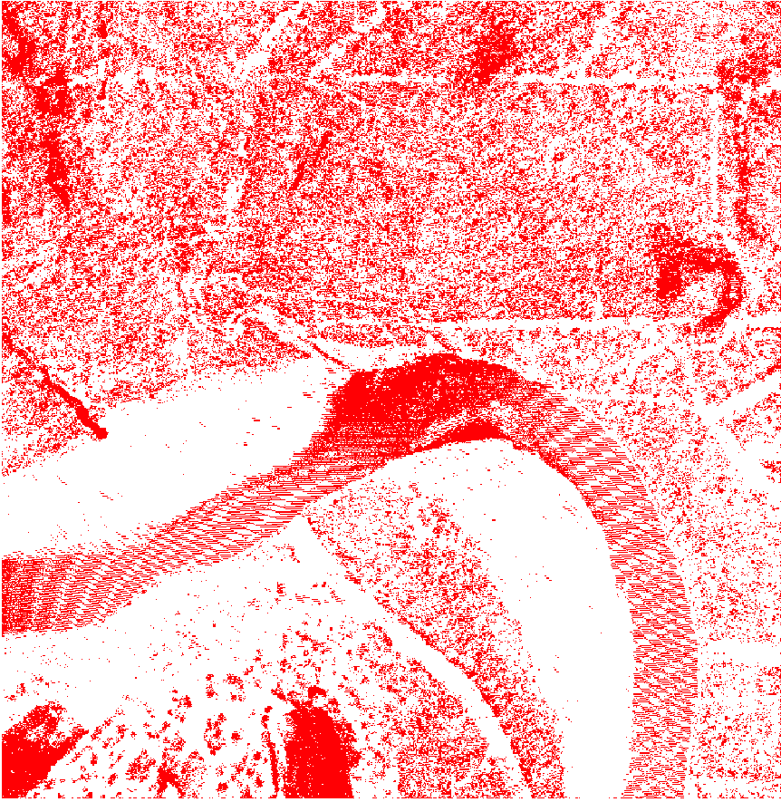
STATISTICS_STDDEV=4.5863482236128The image below is the LiDAR density raster that has been reclassified to only the cells that do not have any point measurements for that area. This is important for two reasons. First, we see what areas of the terrain are not returning any LiDAR points so we can get a sense of where the DEM might be less accurate. Second, we can use this visualization to adjust our DEM resolution to ensure there are an adequate number of LiDAR points per raster cell throughout the study area.
Step 4
Convert .las to GeoPackage
In order for a DEM to be created from LiDAR points we have to convert the data from .las format to GeoPackage format. This step is the most computationally intensive process and will require some additional hard drive space as the GeoPackage format does not store the point cloud as compactly as LAS. For example, the point cloud used for this tutorial is 650 MB in size in .las format and is 808 MB. This could partially be due to the fact that a topology is built during the point cloud import and is also likely why the process is computationally intensive. This does make sense in the long run as future calculations will be a lot more efficient once the GeoPackage is created.
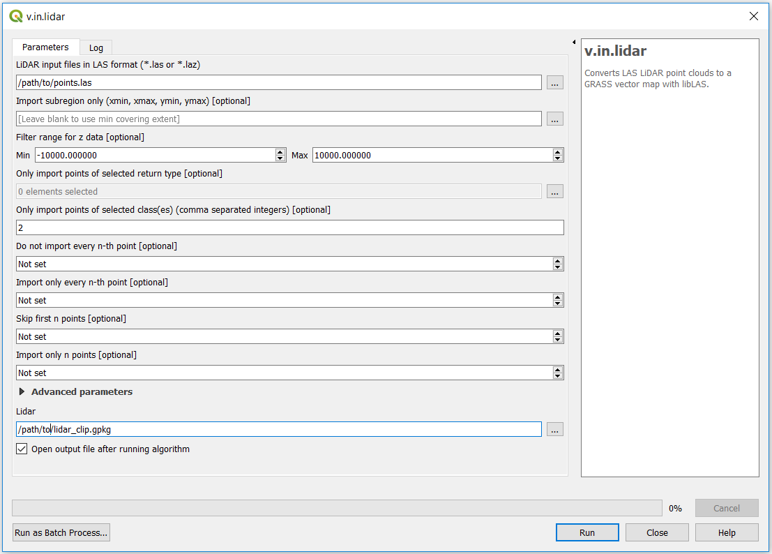
Import point cloud with v.in.lidar
In your open QGIS project search for v.in.lidar in the Processing Toolbox panel or browse for it under GRASS -> Vector (v.*) -> v.in.lidar. There are input parameters that are key for the import. First is the Filter range for z data [optional]. This is not optional! If you do not set these values above and below the elevation range of the point data not all of the point data will be imported! Second, Only import points of selected class(es) (comma separated integers) [optional] should be set to 2 to only import the ground classified point. The rest of the parameters can be left as default (see image below).
Step 5
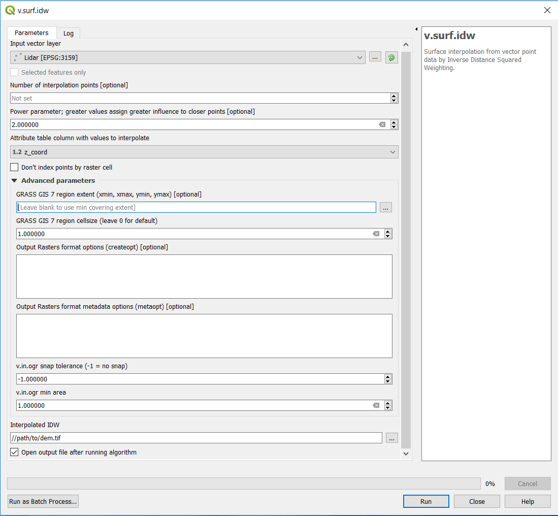
In this step we will use the GRASS GIS v.surf.idw tool to create a DEM. We know from the statistics performed in the previous steps that the majority of the cells have enough point readings per cell (~4) to use a 1 meter resolution for the DEM. Also, because the points are irregularly dispersed across the study area and there are significantly sized areas that do not have elevation readings, we will use a mathematical method called Inverse Distance Weighting (IDW) to calculate an appropriate elevation value for each raster cell. GISGeography is an excellent resource for understanding how IDW works.
There are several parameters that can be tweaked to affect the resulting DEM depending on what the data will be used for. The most significant variable is the Power parameter. A higher power will increase the weight of elevation points closer to a given cell meaning better accuracy for cells with lots of LiDAR points close by but results in a much rougher surface. A lower power will result in a smoother surface which might be contagious when producing hillshade rasters and surface flow models.
The next key parameter is cell size. The resulting DEM will likely be the base for lots of future analysis and models, so the cell size must be chosen carefully to try and find the balance of highest possible resolution, processing demands, project scale and accuracy demands. A 1m resolution is quite common and is flexible in that it can be down sampled to a lower resolution later and is appropriate for most industries.
The parameters to generate a good all round DEM can be seen in the image below. The key parameters that were changed from the default values are:
Number of interpolation points:Delete Default value of 12 leaving value of "Not Set"
Attribute Table Column with values to interpolate:z_coord
GRASS GIS 7 region cellsize:1 *This is the resulting raster cell size
Step 6 - Validate Results
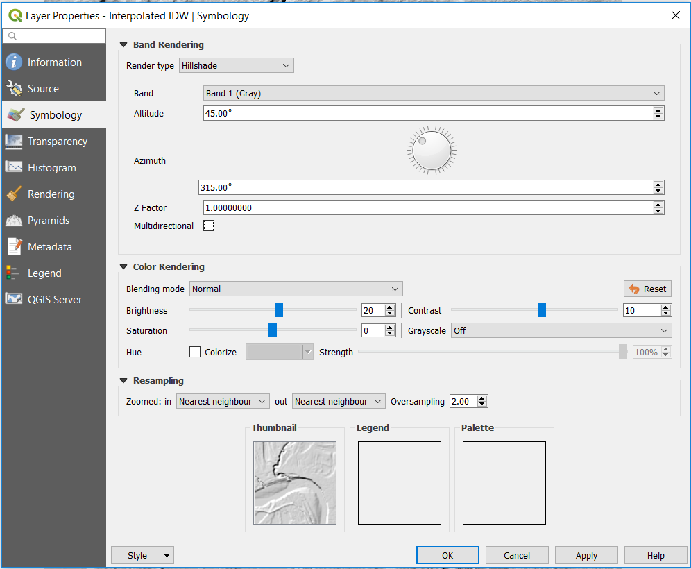
The final step in the process is to validate the DEM. To do this we will generate a Hillshade visualization from the DEM which will help to get a sense of the terrain, make any obvious errors such as not selecting the proper return type (trees make the hillshade look very rough) and will verify there are no gaps in the data.
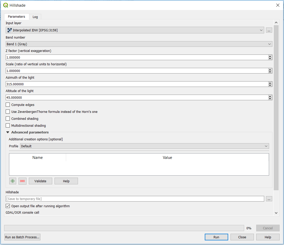
With QGIS there are a couple of quick and easy ways to visualize the DEM as a hillshade. One way is to change the symbology of the dem from gray scale to a rendering type of "Hillshade" (See first image below). The second way is to generate a new Hillshade raster by clicking on the Raster toolbar at the top and in the dropdown menu select Analysis -> Hillshade.... The parameters can be viewed in the second image below.
Conclusion
Through this tutorial you should now be able to create a DEM from LiDAR using QGIS with GRASS modules and validate the data by generating a hillshade raster. This DEM can be used as base data for a wide array of models and calculations such as viewsheds, watershed, slope, terrain ruggedness, least cost paths and much much more!
The ability to perform these advanced GIS procedures using free and open source software is truly amazing. Hopefully you found this tutorial easy to follow. The final hillshade can be viewed in the interactive map below.
If you have any questions or comments please feel free to create an account or safely and securely sign in with your Facebook, Twitter or Github account.
On June 28, 2023, 7:17 p.m. GIS_student says:
Where is the vector lidar file coming from in the Step 5 GRASS GIS v.surf.idw tool?