Managing fresh water and the watershed areas they flow in is becoming an increasingly important issue for industry and government. A watershed is essentially a collection area for groundwater flow that is determined by the surrounding terrain and heights of land. Understanding the boundaries of the watersheds and the locations of the stream channels can help developing policies, development plans and industry partnerships for these areas. This proposed project, with the support of the City of Prince Rupert will use precise high resolution elevation data to create a watershed model for the Woodworth Lake area to the northeast of Prince Rupert. Benefiting from this project will be the City of Prince Rupert who will receive digital products representing the Woodworth Lake watershed area and myself who will gain valuable professional experience carrying out the GIS procedures.
***NOTE*** This web page uses WebGL technology that may only work in Google Chrome at this time. Some of the interactive content is
dependant on WebGL so using the Google Chrome web browser is highly reccomended.
The sponsor for this project is the City of Prince Rupert who serves a community of 12,000 citizens.
This is a port town located in mountainous Northwestern British Columbia (54.27°N, 130.37°W) that provides a wide variety of municipal services
to its residents including development services, public works, emergency services, recreation and, uniquely, services of ferry transportation to
the airport.
Rheannon Brooks was the project supervisor providing guidance and feedback throughout the project. Communication with Rheannon was a key factor
for the success of this project. Rheannon was able to provide additional data and local knowledge that allowed for the generation of watershed
product that the city can use in planning of future projects in the maintenance and monitoring of their watersheds.
The following video, published by the City of Prince Rupert, provides a little bit of the background of the significance of the Shawatlan and
Woodworth Lakes, which is where the primary area of analysis is.
Project Background
Personal Interest
Using LiDAR to delineate stream networks and watershed boundaries is an interesting project to me as it expands on my original interest in utilizing LiDAR in archaeology for identifying archaeological sites. I am fascinated by the ability of LiDAR to penetrate through forested areas creating dense point cloud representations of underlying terrain but also buildings and vegetation above it. Also, my previous work in the forest industry where part of our cut block planning included mapping, measuring and protecting streams. This project will be able to combine my interests and past experience.
Project Purpose
The purpose of this project is to create digital products that will help in the management and planning of the watershed areas surrounding Woodworth Lake. The identification of these boundaries will allow the City of Prince Rupert to identify how industry and the public are or could impact the watershed and will allow them to create strategies to manage the watershed with these parties.
Benefit to Industry
This project will be a benefit to industry and to the public in general because a highly accurate and current model of the watershed area will be created. This will save money and time in the early stages of project planning in these areas and will allow for early mitigation to impacts to the watershed areas.
Beneficiaries
Because of the increasing value of fresh water this project will have benefits to a wide range of beneficiaries the most important being the environment. Protecting watersheds and ground water flow will also be very beneficial to the greater public and the City of Prince Rupert aiding in the planning of a sustainable future.
Software
Processing high resolution, high precision LiDAR point clouds and creating elevation, stream and watershed GIS products requires sophisticated, powerful, robust and efficient software.
There are relatively few options to choose from when deciding what software to use, especially when you take the following considerations into account:
LiDAR/Point Cloud Processing
Raster Processing
Geoprocessing Modeling
Stream Calculation Tools
Watershed Calculation Tools
Map Display
It is essential to find a software that encompasses all of these items. When conducting big projects many hours of coding, processing and troubleshooting can be saved with the right software.
This extension allows ArcGIS for Desktop to work with LiDAR point data.
Through this project I was able to examine some of the software options. Below is a table listing the costs and benefits to using ESRI's ArcGIS Desktop (paid) software and also QGIS and GRASS GIS (free/open source) software.
Software Comparison
Software Function
ESRI/ArcGIS Software
Open Source Software
(PDAL, QGIS, GRASS GIS)
LiDAR Manipulation
The LiDAR dataset provided from the City of Prince Rupert was customized for use in ArcGIS, as such it was easy to import into the system.
To do this you must create a las dataset based on a selection of LiDAR files and then a LAS Dataset Layer is created where the ground returns
can be isolated. In order to do this the 3D Analyst extension is required, which adds to the expense as all of the other processing is done with
the Spatial Analyst Extension.
Importing the LiDAR data into GRASS GIS was initially complex because the point cloud data was segmented into 1 km2 las files. The processing time
and scripting required to import all of the files was not practical which necessitated the use of the Point Cloud Data Abstraction Library (PDAL).
This proved to be convenient as PDAL can quickly extract ground returns and merge las files leaving it in a state that is easily imported into GRASS.
The import into GRASS is done with one tool that takes significantly longer to run that the ArcGIS process as it needs to convert the las into GRASS
Points while simultaneously creating a topology. This takes several hours where ArcGIS only takes half an hour.
DSM Extraction
To create a DSM raster to begin the analysis several tools must be run. ArcGIS tends to create odd edge artifacts that nictitates extra processing
to create a polygon representing the boundary of the LiDAR data that then clips the edge of the DSM to ensure accurate results. Also, because the
LiDAR data did not have the Spatial Reference built into the file headers, the resulting outputs needed the Spatial Reference to be set.
The DSM is altered in this phase to remove lakes as only parts of the lakes had LiDAR coverage and calculating stream flow through lake areas is
impractical.
Creating a DSM with GRASS GIS was quite easy. Only one process was required and it ran very efficiently. The methods for determining raster cell values
based on the point data was similar to ArcGIS in that they both use similar terminology for the interpolation methods. A difference is that GRASS GIS
has a specific tool for each interpolation method and ArcGIS allows you to select the interpolation method of choice in one tool (LAS Dataset to Raster).
Stream Modeling
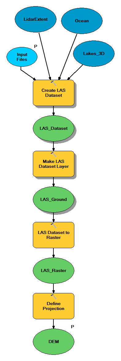
The stream modeling process in ArcGIS requires a large array of processes (see Figure 3). The ordering of these tools was quite challenging and
took some trial and error to get the tools to link up. The least intuitive part of this process was the need to use the “Con” tool to which determines
how much flow accumulation a raster cell needs before it is considered to be a stream cell.
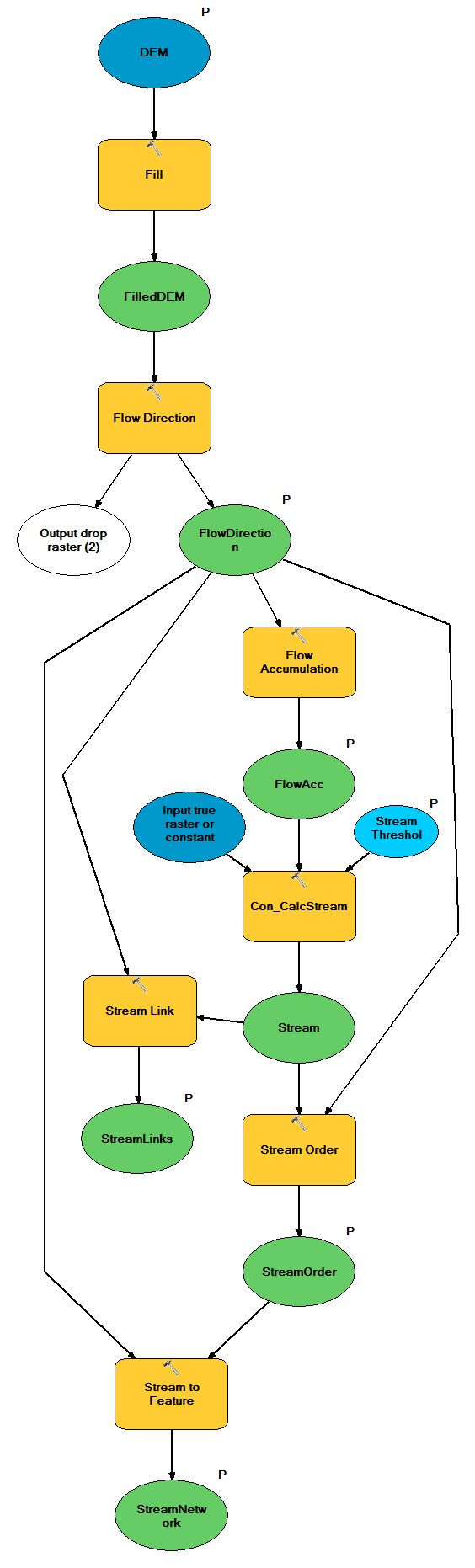
GRASS GIS required only two tools to create stream vectors. It took some research to determine the tool required to initiate the process (r.terraflow).
This tool outputs all the rasters required to calculate stream networks (see Figure 4). One significant limitation of GRASS is its ability to determine
stream order. The tool used to calculate stream order is r.stream.order which worked well on the test area; however, when used on the full Woodworth Lake
area, the computer quickly ran out of RAM and the process stalled. This was tested with 16 GB of RAM.
Watershed Modeling
To generate the watersheds with ArcGIS, a significant amount of python scripting was required. A selection process was required to find the ends of all
stream segments that terminated on a lake or ocean and at the junctions of higher order streams as determined by the user. An iterative process was
then used to calculate a watershed area for each pour point.
Due to the inability to calculate stream order I did not execute this step. It is possible to calculate watersheds based on sinks,
but I wanted to calculate watersheds based on certain stream order junctions, so this was not possible.
Map Display
ArcGIS is the industry leader for not only geoprocessing but for mapping/cartography. As such, it is easy to create map displays for the meetings and
demonstrations.
In the time that I started this project a significant QGIS software release came out (QGIS3). This significantly updated software made creating map
layout for sharing and demonstrations easy. It even allowed for 3D visualization that enabled me to get a good sense of the terrain around Woodworth Lake.
Data
Layer Name
Feature Type
Attribues
Value
Description
LiDAR
Full Feature Point cloud (.las)
Return Type Classification
2
Ground
3
Low vegetation
4
Medium vegetation
5
High vegetation
6
Buildings
9
Water
Cadastral Land Parcels
Polygon
Legal Description
String
Location Description of Parcel
Ownership
String
Private or Crown land
TRIM Streams
Line
Name
String
Stream Names
Orthophoto
Raster (ECW)
RGB/ 10 cm Resolution
RGB
Color Orthophoto
Lakes
Polygon
Name
String
Lake Name
DataBC Coastline
Line
Length
Double
Line Length
Woodworth Lake GDB (Deliverables)
Vector Data
StreamNetwork
Line
stream_id
Intiger
Unique ID for joining other tables
stream_order
Integer
Stream Order. Larger number = larger stream
PourPoints
Point
pour_id
Integer
Unique ID for joining other tables
stream_id
Integer
Field for joining to streams table
stream_order
Integer
Stream Order
Watersheds
Polygon
watershed_id
Integer
Unique Watershed ID
pour_id
Integer
Field for joining to PourPoints table
stream_order
Integer
Stream Order
Raster Data
DEM
Raster
Elevation
Double/1m Resolution
LiDAR derived elevation
DEM_Filled
Raster
Elevation
Double/1m Resolution
Elevation raster with sinks removed
FlowAccumulation
Raster
Flow Accumulation
Integer/1m Resolution
Cell value represents total number of cells flowing into that cell
FlowDirection
Raster
Flow Direction
Integer/1m Resolution
Cell value represents total number of cells flowing into that cell
Surface constraint created from digitizing built up areas. Used as a "Hard Erase"
Culvert
Polygon
elevation
Double
Surface constraint created from digitizing anticipated culvert locations. Usually 3m wide. Elevation field represents the elevation to be burned into the raster in order to relieve signficant sinks along high grade roads.
LidarFootprint
Polygon
OBJECTID
Integer
Extent of the point cloud used to force DEM to follow point cloud coverage by using it as a "Hard Clip" surface constraint. The extent is calculated in a separate model.
StreamNetwork
Line
stream_id
Intiger
Unique ID for joining other tables
stream_order
Integer
Stream Order. Larger number = larger stream
PourPoints
Point
pour_id
Integer
Unique ID for joining other tables
stream_id
Integer
Field for joining to streams table
stream_order
Integer
Stream Order
Watersheds
Polygon
watershed_id
Integer
Unique Watershed ID
pour_id
Integer
Field for joining to PourPoints table
stream_order
Integer
Stream Order
Raster Data
DEM
Raster
Elevation
Double/1m Resolution
LiDAR derived elevation
DEM_Filled
Raster
Elevation
Double/1m Resolution
Elevation raster with sinks removed
FlowAccumulation
Raster
Flow Accumulation
Integer/1m Resolution
Cell value represents total number of cells flowing into that cell
FlowDirection
Raster
Flow Direction
Integer/1m Resolution
Cell value represents total number of cells flowing into that cell
Working with large volumes of LiDAR is very processing intensive and time consuming. In order to increase processing speed and reduce errors
the full feature LiDAR tiles were manipulated with PDAL so that there was only ground and water classified returns in the data, the tiles were
grouped into the three geographic areas this project was broken down into and a spatial reference was added into the header information to ensure
there were no projection errors.
PDAL was used to combine, select ground and water returns and assign a projection to the las files. The PDAL JSON pipeline is shown below.
The pipeline was then executed with commandline feeding the files into the pipeline
setlocal EnableDelayedExpansion
set js_files=
for %%f in (*.las) do set js_files=!js_files! %%f
echo %js_files%
pdal pipeline -i assign_srs.json --readers.las.filename=%js_files% --writers.las.filename=.\srs\merged.las
PDAL pipelines also make it possible to clip LiDAR into smaller sections that can be used for exploring the point cloud and getting a
better sense of the terrain in certain areas. The point cloud on the right was used to help find where culverts should be placed to allow
streams to flow across the highway.
ArcGIS DEM Model
GRASS GIS DEM Model
Elevation Surface (DEM) Creation
The first step in modelling streams and watersheds from point cloud format is to create a
Digital Elevation Model (DEM) raster.
From a DEM, it is possible to create all of the prerequisite data for watershed modeling.
There are some important considerations that must be taken into account when creating a DEM for watershed analysis. First, a very large area
will be processed, so to improve efficiency, it is important to choose a processing cell size that is as accurate as possible but also not at
too high a resolution that it will cause the processing time to take too long or to cause memory issues. For this model a cell size of 1 meter was used giving us
most optimal resolution and accuracy.
Second, in some terrain, there are man made features that will alter the way ground water flows that can not be detected by LiDAR. Culverts and
bridges are the most common features in open terrain that need to be accounted for. These structures are on top of the groundwater flow, so in order to minimize the flow errors created by these structures
they need to be "burned" into the DEM with elevation values that represent the height of the stream channel or culvert which should remove artificial SINKS.
Ideally the locations and heights of these structures will be collected with high accuracy GPS or survey, but one of the limitations of this project is
that all of this information had to be inferred from the elevation data or the orthophoto.
Third, the LiDAR dataset for this project did not include significant portions of the lake area which required the elevation of the lake to be placed into the DEM
as a 'Hard Replace' surface constraint to allow the flow accumulation to build across the full catchment area.
The modelling process for creating a DEM can be seen on the right as built in ArcGIS Model Builder and GRASS GIS.
ArcGIS DEM Model
GRASS GIS DEM Model
Stream Modeling
Modeling over ground stream flow requires many different rasters to be calculated, combined and converted. The first step is to ensure there are no
obstructions in the stream flow. This was partially considered when surface constraints were added in the DEM creation process, but you must also
ensure that each cell of the raster can flow all the way to a major sink, such as a lake, or to the edge of the study area. This can be accomplished
by "Filling" the DEM to remove flow errors. From this "Filled" DEM, a flow direction
for each cell is calculated. This raster will be the basis for all
of the subsequent calculations.
From the flow direction raster a flow accumulation
raster is calculated which is important for determining where a stream will be initiated. This determines how many cells are upstream of any given
raster cell. Then, to calculate the streams a condition is applied to the flow accumulation raster where if the flow accumulation value of a cell is below a given
number it will be given a NULL value resulting in a raster with cell values that represent streams. For this project, streams were initiated at a flow accumulation
threshold of 1000 cells.
  # Calculate Streams based on flow accumulation threshold (user determined)
  arcpy.gp.Con_sa(FlowAccumulationRaster, 1, StreamRaster, "", 1000)
For the purposes of this project a Stream Order calculation
was performed on the stream raster using the Strahler method. The stream order will later be used to calculate the location of pour points.
The tools required to calculate streams are displayed to the right. You can see the large number of processing tools that are required to create a stream vector in
ArcGIS. GRASS GIS uses relatively few tools to create the same outcomes.
LiDAR Streams vs. TRIM Streams
The adjacent map compares the resolution, stream density and accuracy between the vector streams calculated from a 1m resolution DEM
in this project and the TRIM streams calculated at a 1:20,000 scale available from a provincial dataset. TRIM
is the most authoritative data that is available province wide that contains topographic information such as streams, lakes, roads, utilities,
contours and a wide range of other information.
In this Swipe Map, the thicker and darker blue lines represent the TRIM streams and the lighter and thinner blue lines represent the streams calculated
in this project.
Swipe the vertical bar in the middle to compare the difference in the streams.
Watershed Modeling
The procedure for calculating a watershed area is quite simple. First, a pour point is selected, usually as a vector point. That point is then
superimposed on the flow accumulation raster, snapping it to the highest flow accumulation value within a selected distance. The Watershed Tool is then
run using the snapped pour point and flow direction raster as input. The tool then determines the area that flows into that point. The resulting watershed
raster can then converted into a vector polygon for analysis and map display.
A major challenge for this project was creating an algorithm that automatically selected and snapped pour points to base watershed areas on. This is challenging
to do for a large area because when the Watershed tool is run, if there are any overlapping watershed areas, such as multiple pour points along a stream, only portions
of those watersheds will be captured in the results because rasters can only have one value per cell. This means it is very difficult to run pour points in batch, unless
there is only 1 pour point per connected stream network. Generally, this is not an issue as most watersheds are calculated at the ends of stream networks where the stream
either encounters a lake, shoreline or the edge of the processing area. The method the City of Prince Rupert chose required multiple pour points along higher order streams,
thus requiring a custom algorithm to be made.
Custom Watershed Algorithm
The City of Prince Rupert required that watershed areas be determined from the end points of streams with a stream order of 3 or greater.
The first step in creating the custom algorithm was to write a python script to determine the end points of streams that were at a certain stream order or higher.
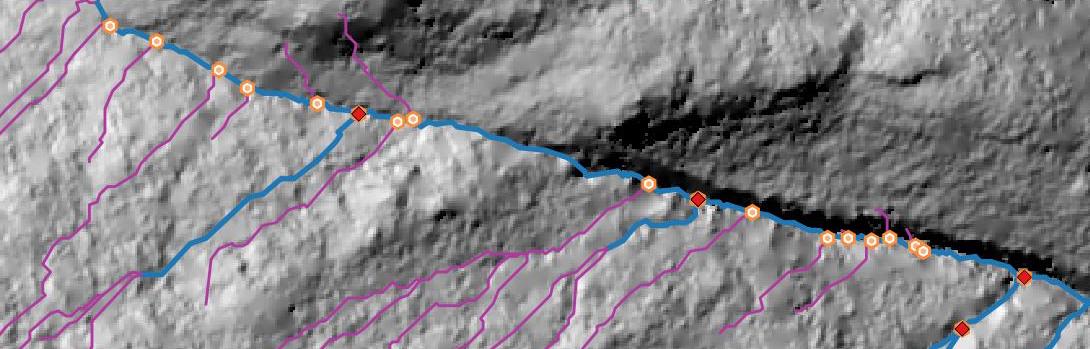
This was a challenge because all of the streams were segmented when one stream intersected another (see image below). This meant that it was not possible to simply calculate a start
or an endpoint for any one particular stream (unless it was a first order stream). So, in order to calculate the pour points the end point of all stream segments of
a stream order of 3 or higher was calculated.
#Problem Solving
Pour Point Identification (above image)
In the above image the thick blue lines represent the higher order streams that the pour points need to be calculated for. The purple streams
are the lower order streams that cause the higher order streams to be segmented at the intersections leading to the orange pour point symbols
that result when trying to find the end points of the higher order streams. The custom algorithm below was written to find the final pour points that are shown in the image.
Algorithm Step 1:
Create Pour Point Featureclass with same fields as Stream Featureclass
#Parameters for creating a new pour point feature class
out_path, out_name = os.path.split(str(PourPoints))
geom = "POINT"
has_m = "DISABLED"
has_z = "DISABLED"
spatial_reference = arcpy.Describe(StreamNetwork_FC).spatialReference
#create an empty pour point feature class using the stream feature class as the field template
pour_points = arcpy.CreateFeatureclass_management(out_path, out_name, geom, streams,
                                                  has_m, has_z, spatial_reference)

#Get fields from Stream Featureclass to be used in the insert and search cursors
stream_field_names = ['SHAPE@']
for f in fields:
    stream_field_names.append(f.name)
# Remove shape fields that don't exist in the Pour Point Featureclass
remove_fields = ['Shape_Length']
for r in remove_fields:
    try:
        del stream_field_names[stream_field_names.index(r)]
    except:
        pass
Algorithm Step 2:
Find Stream End Points, Add to Pour Points and remove duplicates
# Select all streams with a stream order equal to or above user selected stream order threshold
exp = u'{} >= {}'.format(arcpy.AddFieldDelimiters(StreamNetwork_FC, "grid_code"), Stream_Order_Limit)
search_cursor = arcpy.da.SearchCursor(StreamNetwork_FC, stream_field_names, exp)
insert_cursor = arcpy.da.InsertCursor(pour_points, stream_field_names)
exisitingPoints = []
for row in search_cursor:
unique = "True"
for point in exisitingPoints:
if row[0].lastPoint.equals(point):
unique = "False"
else:
pass
if unique == "True":
exisitingPoints.append(row[0].lastPoint)
insert_cursor.insertRow((row[0].lastPoint,row[1],row[2],row[3],row[4]))
else:
pass
search_cursor.reset()
for row in search_cursor:
unique = "True"
for point in exisitingPoints:
if row[0].firstPoint.equals(point):
unique = "False"
else:
pass
if unique == "True":
exisitingPoints.append(row[0].firstPoint)
insert_cursor.insertRow((row[0].lastPoint, row[1], row[2], row[3], row[4]))
else:
pass
del search_cursor, insert_cursor
Algorithm Step 3:
Use Lower Order Streams to Select Unwanted Pour Points and Delete
#Temp feature class used to select excess pour points
temp_streams = arcpy.CopyFeatures_management(stream_clip,'in_memory/temp_streams')
temp_streams_fc = arcpy.MakeFeatureLayer_management(temp_streams, "temp_streams_fc")
pour_points_fc = arcpy.MakeFeatureLayer_management(pour_points,'pour_points_fc')
exp = u'{} >= {}'.format(arcpy.AddFieldDelimiters(temp_streams_fc, "grid_code"), Stream_Order_Limit)
delete_cursor = arcpy.da.UpdateCursor(temp_streams_fc,'*',exp)
for row in delete_cursor:
delete_cursor.deleteRow()
del delete_cursor
arcpy.SelectLayerByLocation_management(pour_points_fc, "INTERSECT", temp_streams_fc)
delete_cursor = arcpy.da.UpdateCursor(pour_points_fc,'*')
for row in delete_cursor:
delete_cursor.deleteRow()
del delete_cursor
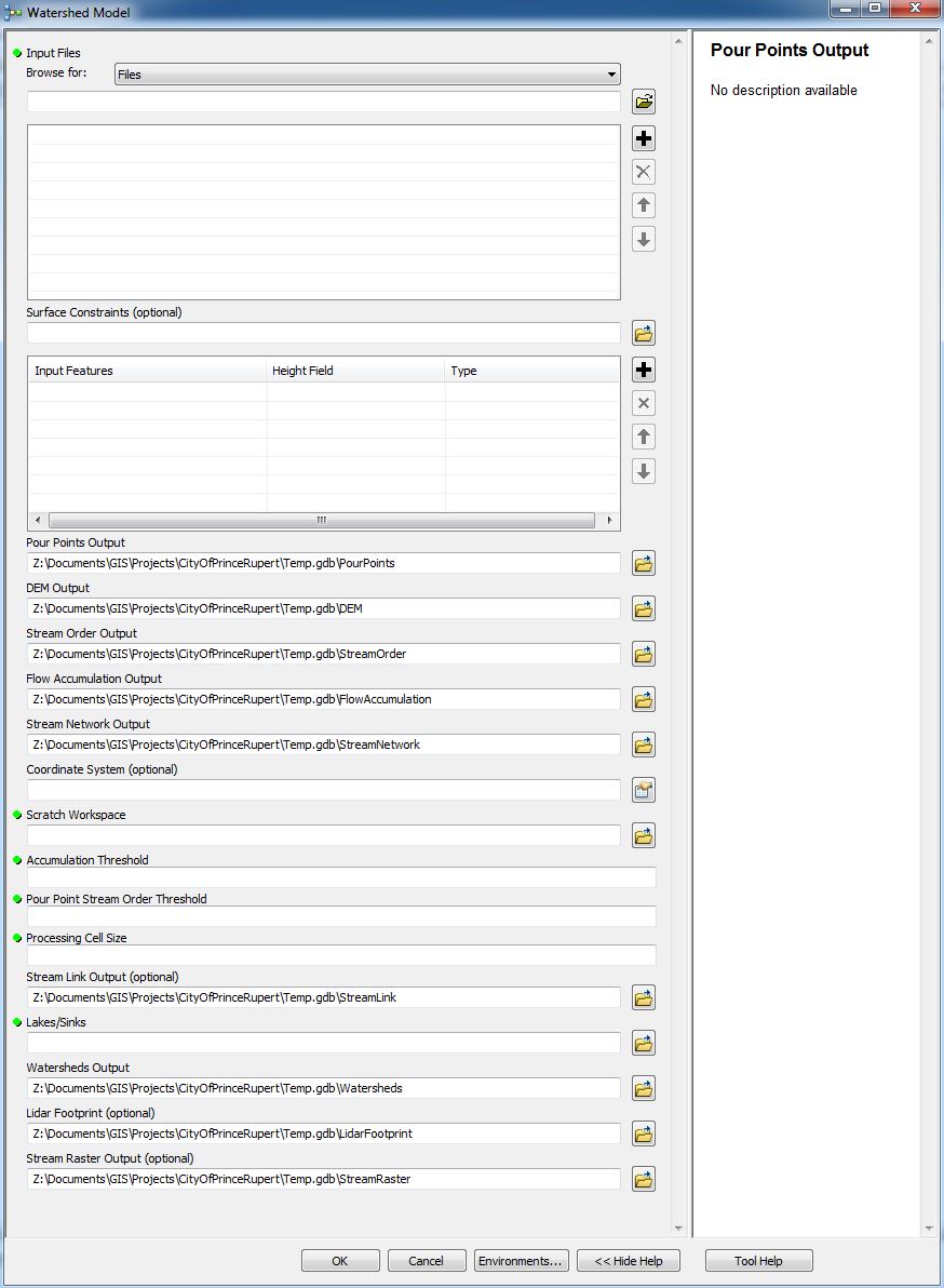
Using the python programming language and ESRI's arcpy python GIS library was essential for the success of this project. The use of scripting tools allows
for set processes and parameters to be run on the data producing consistent results. It also allows for custom tools to be build making the process user friendly
and efficient for use in the future and across organizations.
From the onset of this project the tools and parameters used in the processing and caluclations were executed with python script. Without the ability
do these specific calculations it would not have been possible to meet the needs of the City of Prince Rupert. Utilizing these scripts also saved hours of processing time
while simultaneously documenting the processing steps and allowing flexibility in what parameters can be entered. The tools and script was developed on the Woodworth Watershed
and then was extended to cover Kaien Island and Digby Island.
In the end it was possible to turn the script into a tool that the City of Prince Rupert can use in the future to recreate the results or to adjust some of the key parameters.
CUSTOM WATERSHED CALCULATION TOOL
#Problem Solving
In order to conduct some of the specialized procedures for the geoprocessing required for this project, a custom python script was written that
allows for customization of the parameters used to create the watershed products so that it can be applied to other areas in the future.
One major issue in creating this tool was the ability to include surface constraints that would be incorporated into the LiDAR/DEM processing.
The input parameters must include 3 parts: the surface constraint feature class, a list of each feature class’ fields and a set list of surface
constraint types.
This is challenging because it is not known what fields are in any given surface constraint and the user must be able to identify the field that
includes the elevation information. After some extensive research and trial and error, it was determined that the only chance at doing this would
be through a python toolbox using a GPValueTable as the parameter input. Using ESRI documentation and trial and error I found that there was no
obvious way to expose the filter list object contained within the GPValueTable such that I would be able to create a new list for each individual
feature. I am sure it is possible but due to time constraints I needed to find a quick solution that would allow for a unified tool to create the
required watershed outputs. This was very important because the process takes several hours to run and had to be iterated many times for each area to
meet the needs of the City of Prince Rupert.
In the end my work around was to create a ArcGIS model builder tool with the python tool added to it, letting the model builder create the LiDAR
dataset with the surface constraints which can be exposed as parameters and run through model builder. The script can be bundled and sent as one
package now, although it takes longer to run and enter parameters relative to running it purely as a python tool.
Conclusion
The Watershed Analysis project conducted for the City of Prince Rupert utilized high density, high accuracy LiDAR information to produce
stream and watershed GIS products that will be used in future analysis and planning by the city.
These products included:
Stream Line Vectors
Watershed Area Vectors
Pour Point Vectors
DEM Rasters
Flow Direction Rasters
Flow Accumulation Rasters
Stream Order Rasters
Stream Link Rasters
Custom Watershed Geoprocessing Tool
Through this project ArcGIS and GRASS GIS combined with other open source GIS tools were explored to find possible more cost effective alternatives
for processing LiDAR and for creating watershed GIS products. Through this we found that it is possible to use open source options with some requiring
fewer processing steps relative to industry leading ArcGIS. However, ArcGIS' ablity to easily create custom tools that can manipulate geometries within
feature classes for customize results and its far more efficient processing of large data sets made it the software of choice for this project.